Bivariate analysis
Interpret the results by answering the following questions:
- Plot each of the two stocks against the market index on a scatterplot. Include these scatterplots in your submission. What are the expected correlations that might exist between each of the stocks and the market index?
- What are the calculated correlation coefficients? Compare these to your plots. Were your initial expectations correct?
- Comment on the coefficients of determination. Which of the two models has the higher explanatory power?
- What are the beta coefficients for each of the two stocks?
- Suppose you were to purchase one of these two stocks, and your decision relied on their volatility in relation to the market index (i.e. their beta coefficients); which of the two stocks would you purchase if you were interested in buying a volatile stock?
From the provided data, the explanatory variable can be described as a stock index. The response VAriables in the current research can be described as Stock 1, and Stock 2.
The developed scattered plots of the provided data are shared below.
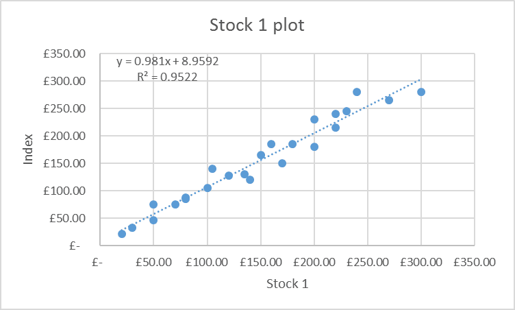
From observing both of the graphs, it can be analysed that both stock values are in great correlation with the index. This is because most of the determined values of Stock 1 are very much close to the trend line. In the stock 2 plot, the determined values are somewhat close to the trend line developed.
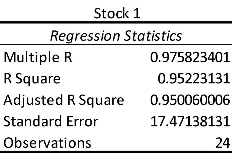
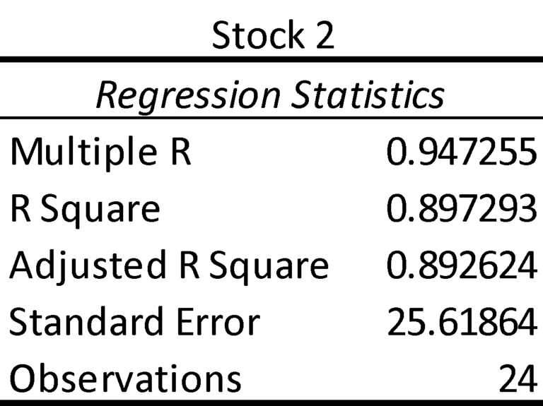
The calculated coefficients of correlation for Stock 1 are 0.9758. The calculated coefficient of correlation for Stock 2 is 0.9473. The calculated values of the correlation coefficient affirm the expectation made from the study of the scattered plot.
The coefficient of determination is the value of R2. From the developed graph of Stock 1, the value calculated for R2 is 0.9522. The value of R2 for Stock 2 is 0.8973. The Stock 1 model in the model with high explanatory power.
Beta coefficient for Stock 1 is equal to 0.98. Beta coefficient for Stock 2 is equal to 0.95
With respect to determined Beta, the most volatile stock to make a purchase for is Stock 2.
Multivariate analysis
Copy the dataset under the second tab, labelled “Question 2”, into a new Microsoft Excel workbook.
Sales figures are usually related to more than one variable, whether it is marketing expenditure, advertising material, shelf placement, or product pricing structures. In this question, total sales figures were found to have a correlation with marketing expenditure and the price of the product. Logically, it could be argued that an increase in marketing expenditure should result in an increase in sales. Similarly, an increase in product price could reduce sales figures.
Using the data provided, perform the following analysis:
- Determine the explanatory and response variables.
- Run a multivariate regression analysis on all three variables.
Interpret the results by answering the following questions:
- What is the calculated correlation coefficient? Do the sales figures correlate with the marketing expenditure and price?
- Comment on the coefficient of determination. What percentage of the response data can be explained by the explanatory variables?
- Determine the multiple regression line equation in the form:
sales^ = (intercept) + (coefficient)× marketing + (coefficient)× price
- Using the regression equation formulated, what is the amount of expected sales (in pounds), if the price is set at £3.50 and the amount spent on marketing is £300?
- Interpret the variables in the regression equation. What impact does each of the factors (marketing and price) have on the sales figures?
The explanatory variables are the price of product and marketing expenditure. The response variable is the sales figure.
The calculated multivariate regression summary of the values is shared below.
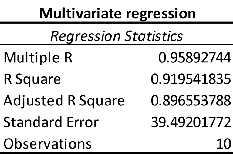
The calculated correlation coefficient for all three variables is shared below.
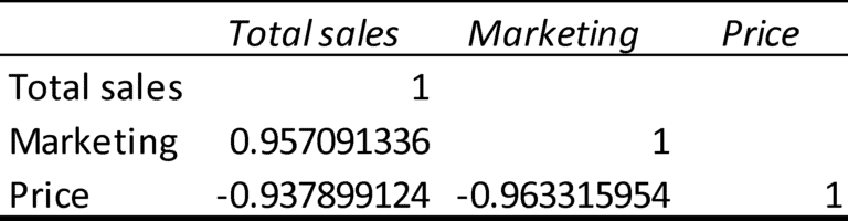
From the above table, it can be discussed that sales figure have a positive correlation with the marketing practices with the value of 0.9571. Whereas, sales value has a negative correlation with price with the value of -0.9379.
The coefficient of determination (R2) explains the level of variation between the dependent variable (sales) and independent variables (marketing expense, and price of the product). The value of R2 is 0.9195, that explains that variation in the dependent variable is due to change in the independent variables.
Sales = 6.83 + 0.265 (marketing) + 0.22(price)
From above developed equation, the amount of expected sales will be as follows:
Sales = 6.83 + (0.265*300) + (3.5*0.22)
Sales = 6.83 + 79.5 + 0.77
Sales = £87.10
The chosen variables for the developed regression equation are based on the intercept of 6.83 that explains the sales revenue of the company when they are not producing any product, nor they are doing any marketing activity. Yet, the coefficient of marketing explains the percentage of marketing been performed for the products in a single market with a positive impact. The coefficient of product price describes the level of price having a reduced impact on the overall sales value.